Geometry Is Everywhere — From an Airplane to Relativity

An airplane flies straight ahead

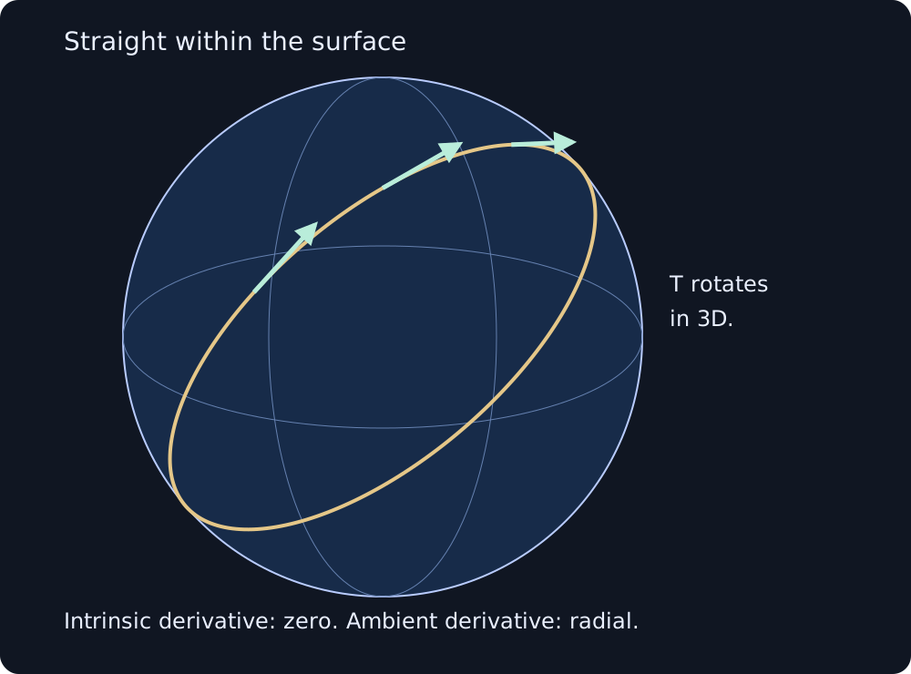
Imagine an idealized airplane constrained to a spherical Earth. Ignore wind, rotation and aerodynamics. Its path follows a great circle: the intersection of the sphere with a plane through its center. What does “straight ahead” mean when the surface itself bends?

Parametrize the path by arc length \(s\), and let \(T\) be its unit tangent. For the sphere's Levi-Civita connection, the geodesic condition is

This does not say that \(T\) is a fixed vector in the surrounding three-dimensional space. With sphere radius \(R\) and outward unit normal \(\hat r\), ordinary differentiation gives

The tangent rotates, but its derivative has no tangential component. Projecting that derivative onto the tangent plane gives zero: no turning within the surface. This is intrinsic straightness. A great-circle segment minimizes length locally, although sufficiently long segments need not be globally shortest. Constant-speed arc length is an affine parameter; an arbitrary change of parameter would add an apparent tangential acceleration.

The Geometry & Invariants experiment makes this distinction visible. Start the flight, reveal the north/east basis, then reveal the components. The numbers generally change even though the tangent is parallel along the geodesic.

What survives a transformation?

There is an elementary precursor in school geometry. Two similar triangles may have different side lengths, yet corresponding angles and ratios of corresponding lengths agree. Uniform scaling preserves those quantities. It does not preserve distances, so a similarity is generally not an isometry.

An invariant always invites a question: invariant under what? Rotations and translations preserve Euclidean distances. Scaling preserves angles but changes areas. A geometric symmetry is a transformation preserving specified structure; choosing that structure determines what counts as a symmetry.

Changing coordinates is another matter. Replacing Cartesian labels with polar labels does not move the triangle or transform its physical shape. It changes its description. The components of a vector then change according to a transformation law, while the vector remains the same object. Coordinate independence is not the claim that every number in every description is invariant.

A physical symmetry makes a further claim about laws or states. Rotating a physical arrangement can produce another allowed arrangement because the laws respect rotations. That is more than writing the same arrangement in rotated coordinates. These ideas connect, but confusing them obscures precisely what a calculation establishes.

A vector belongs somewhere

A tangent vector at \(p\) belongs to the tangent space \(T_pM\). A tangent vector at another point belongs to another vector space. On an abstract manifold there is no automatic identification between them. The familiar act of sliding an arrow without changing it relies on the additional structure of Euclidean space.

A scalar function \(f\) provides a natural way to probe a tangent vector. Its differential is

Repeated indices are summed. The covectors \(dx^i\) form the basis dual to the coordinate vectors \(\partial_i\): \(dx^i(\partial_j)=\delta^i_j\). Thus \(df\) is a linear functional on tangent vectors, giving the directional rate of change of \(f\). It is a one-form, not a vector with decorative lower indices.

A metric can turn a covector into a vector: the gradient satisfies \(g(\operatorname{grad}f,v)=df(v)\). The differential itself does not require a metric. This distinction matters whenever the geometry is not already built into familiar Cartesian notation.

A differential one-form is a smoothly varying covector field. Higher differential forms are alternating multilinear functions of several tangent vectors. A two-form, for example, evaluates oriented infinitesimal area elements. Their transformation and integration rules reflect these geometric roles. They are not simply collections of indexed numbers renamed for elegance.

The basis is changing too

Write a vector field locally as \(V=V^i e_i\). Differentiating its components alone ignores that the local basis may vary. In an embedded surface, even differentiating the full ambient vector introduces normal changes that are not intrinsic changes within the surface.

A connection specifies how to compare nearby tangent vectors. In a coordinate basis \(e_i=\partial_i\), define \(\nabla_j e_k=\Gamma^i_{jk}e_i\). The product rule then yields

The Christoffel symbols are connection coefficients in that coordinate basis. Their extra term records the basis's contribution; it is not an arbitrary correction added to force a desired answer. The symbols themselves do not transform as tensor components. The complete covariant derivative does.

Consider the Euclidean plane in polar coordinates. Its metric is \(dr^2+r^2d\theta^2\). Here \(\Gamma^r_{\theta\theta}=-r\) and \(\Gamma^\theta_{r\theta}=\Gamma^\theta_{\theta r}=1/r\), despite the plane being flat. The coordinate basis changes with position. A connection describes comparison; curvature measures the failure of such comparison around infinitesimal loops to be path independent. Nonzero coefficients alone do not establish curvature. Given a metric, its unique torsion-free, metric-compatible connection is the Levi-Civita connection used here.

Along a curve \(x(s)\), parallel transport means

This is the central distinction: component change need not be geometric change under the chosen comparison rule. With \(V=T=dx/ds\), it becomes the geodesic equation. The airplane is therefore returning the same answer to two apparently different questions: how to go straight, and how to carry its tangent parallel.

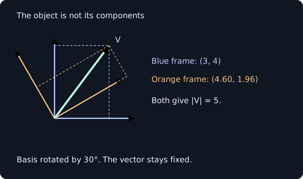
The experiment uses an orthonormal north/east frame, not the latitude/longitude coordinate basis. Let latitude be \(\phi\) and longitude \(\lambda\). Away from the poles, \(e_N=R^{-1}\partial_\phi\) and \(e_E=(R\cos\phi)^{-1}\partial_\lambda\). For \(T=T^N e_N+T^E e_E\), define \(\Omega=\sin\phi\,d\lambda/ds\). Then parallel transport reads

These moving-frame coefficients are not coordinate Christoffel symbols. At a pole, north/east loses its unique meaning; the Cartesian trajectory and its tangent remain smooth. A singular description need not indicate a singular object.

The same language in a different space

Geometry need not describe physical position. For a simple compressible equilibrium system with fixed composition and particle number, take internal energy as a function of its natural variables, \(U=U(S,V)\). Then

This is an equality of one-forms on a thermodynamic state space. Temperature and minus pressure are the derivatives of \(U\) with respect to entropy and volume. Evaluating the one-form on a tangent to a process gives the energy's rate of change along that process.

Because \(dU\) is exact, its integral depends only on the endpoints; around a closed loop it vanishes. For a smooth potential, equality of mixed derivatives implies \(\partial T/\partial V|_S=-\partial p/\partial S|_V\). The identity \(d^2=0\), which yields Maxwell relations in thermodynamics, will reappear in a different physical setting when we formulate Maxwell's equations using differential forms.

Heat and work are generally path-dependent transfers, not state functions with exact differentials. Identifying reversible heat with \(T\,dS\) does not make heat a potential. Legendre transformations offer a systematic change to other natural variables and thermodynamic potentials; that is a later story. Here the point is simpler: the distinction between an object, its arguments and its components remains useful outside ordinary space.

Fields belong to geometry too

In four-dimensional spacetime, the electromagnetic field strength is a two-form \(F\). Locally, in a region admitting a potential, \(F=dA\) for a one-form \(A\). With orientation, metric and source conventions chosen consistently, Maxwell's equations can be written

Here \(J\) is the current three-form, including the coupling constant in this convention; it is not the four-current vector itself. The Hodge star converts a two-form into another two-form in four dimensions using the metric and orientation. Thus the second equation knows about spacetime geometry. The first uses the exterior derivative without a connection, and expresses the homogeneous Maxwell equations in the absence of magnetic sources. Applying \(d\) to the second gives \(dJ=0\), local charge conservation.

This formulation works on curved spacetime without privileging a Cartesian coordinate system. It does not eliminate the metric or the need to calculate components. It places the ingredients where they belong: fields as forms, sources with the appropriate degree, and metric dependence in the Hodge star. See David Tong's discussion of electromagnetic forms for a component construction.

Gravity carries this geometric reasoning further because the metric itself is dynamical. For weak perturbations of Minkowski spacetime, write \(g_{\mu\nu}=\eta_{\mu\nu}+h_{\mu\nu}\) and define the trace reverse \(\bar h_{\mu\nu}=h_{\mu\nu}-\tfrac12\eta_{\mu\nu}h\), where \(h=\eta^{\mu\nu}h_{\mu\nu}\). With signature \((-,+,+,+)\), \(x^0=ct\) and \(\Box=\eta^{\mu\nu}\partial_\mu\partial_\nu\), harmonic gauge \(\partial^\mu\bar h_{\mu\nu}=0\) reduces the linearized Einstein equations to

Here \(T_{\mu\nu}\) denotes stress-energy, unrelated to the airplane's tangent. These are a weak-field approximation, not the full Einstein equations. They resemble the sourced wave equation for the electromagnetic four-potential in Lorenz gauge, \(\partial_\mu A^\mu=0\). The analogy concerns wave operators and gauge freedom; a tensor perturbation and an electromagnetic one-form are different fields. Tong's weak-gravity lectures develop this comparison.

In a vacuum radiation region, transverse-traceless (TT) gauge makes the two gravitational-wave polarizations explicit. Their observable effect is relative tidal motion, described by curvature, rather than an arbitrary coordinate displacement. The humble distinction between arrows and their components has become a distinction between physical geometry and gauge-dependent description.

A coordinate-free formulation does not replace component calculations. It reveals the geometric statement behind the calculation.